
In part 2 of the tutorial, we will show how to get live and historical forex rates into excel by using power query. You will be able to change values in a cell to get updated rates. If you have come across this tutorial for the first time, we recommend reading "Import Currency Rates Into Excel With Power Query - Part 1" first.
Alternatively, you can also read our tutorial on How to Import Currency Rates into Microsoft Excel using our Add-in. The article also accompanies a video.
Let's Begin!
Part I
Step 1
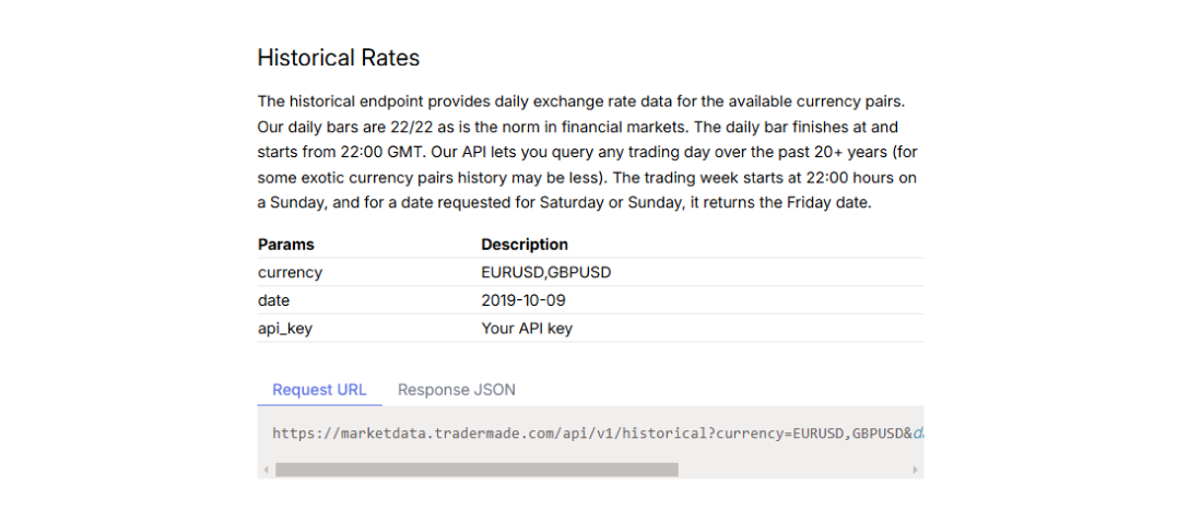
Login to your account and then navigate to the documentation page to copy the URL from the historical rates endpoint, as shown below.
Step 2
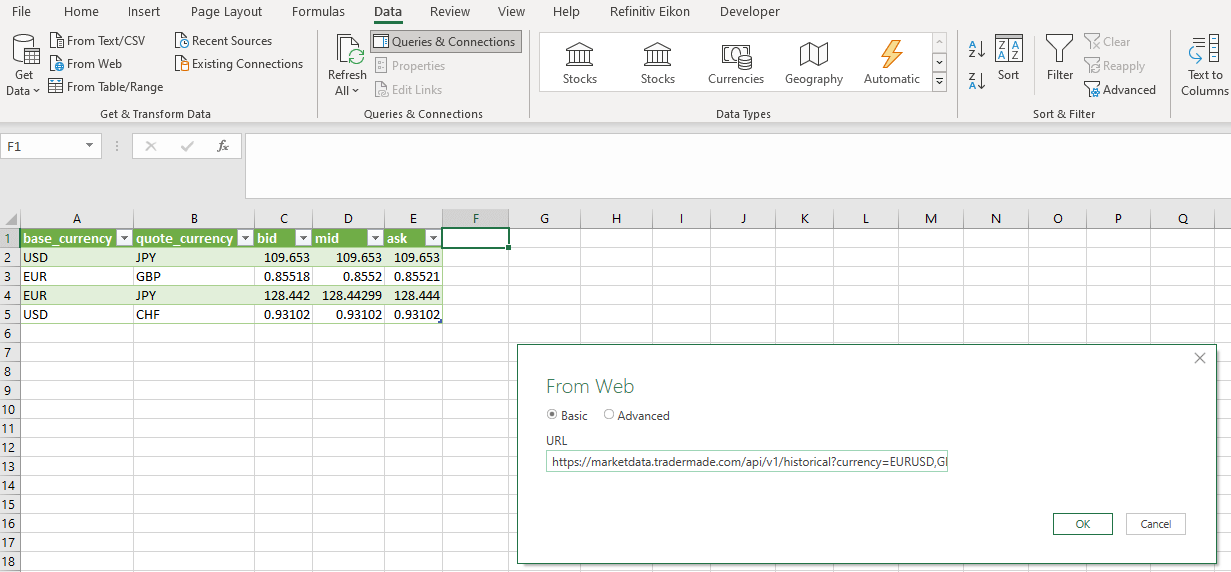
Now Open up an Excel Workbook, and In the spreadsheet, click on the Data tab and then click on From Web (To import data from the web), paste the URL we just copied above as shown below, and click ok. The URL we just copied has three parameters we need to provide to get historical data - two of which we will make dynamic later in the tutorial - first is currencies: EURUSD and GBPUSD; second is date: 2019-10-09 and the third is api_key: your api_key.
Step 3
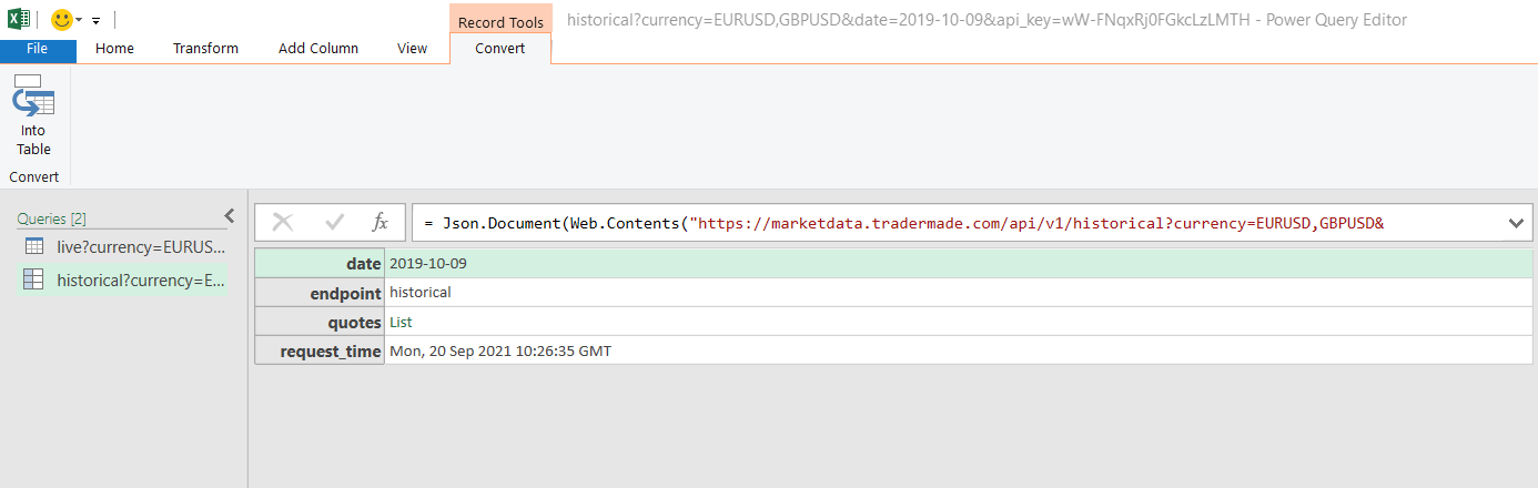
Once you press OK, an editor window will appear; double-click on "List" next to quotes, as shown below.
Step 4
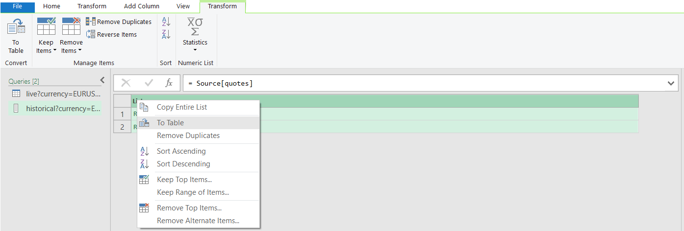
In the Transform window, right-click on the list, click "To Table," and then click OK.
Step 5
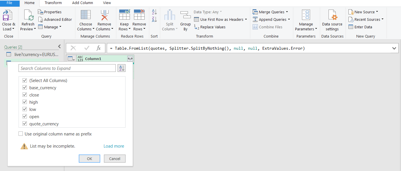
Click on the double arrow button next to Column 1 as shown below and untick "Use original column name as a prefix," and then click OK.
Step 6
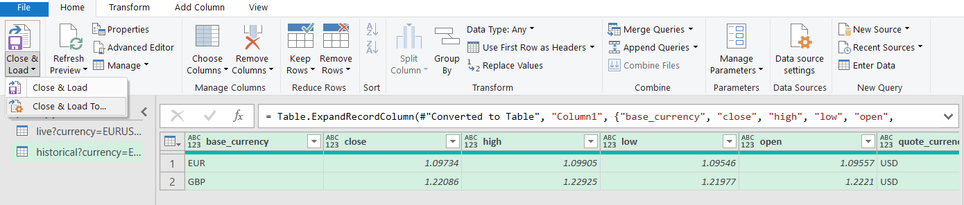
Now press "close & load to" in the top left corner, as shown below.
Step 7
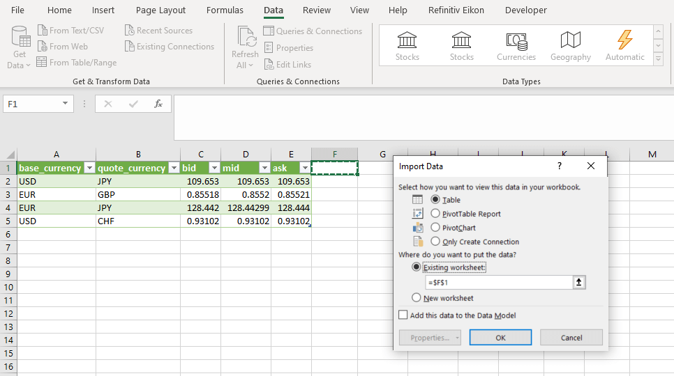
Now select a cell. We choose Cell F1, as shown below, and press OK.
Step 8
You can now see we get historical rates in the cells we want.
Now that we have the data we request, we would like to be able to change cells within the spreadsheet and have the above columns updated. Let's see how to do this.
Part II
Step 9
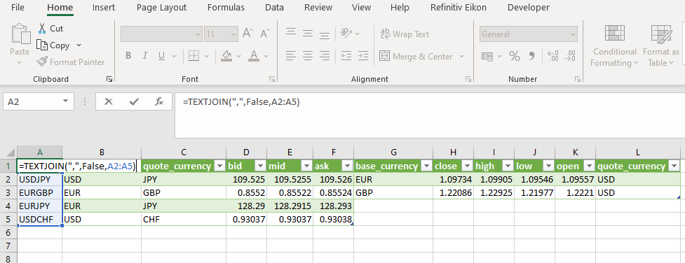
We will insert a new column, as shown below. Then, update cells A2 through A5 with the name of the currencies we want data for. In Cell A1, we will use the function TEXTJOIN(",", False, A2:A5): The formula joins the currency symbols in a format we require to request live and historical forex data. No need to worry; it will be clear how it is used as we move forward.
Step 10
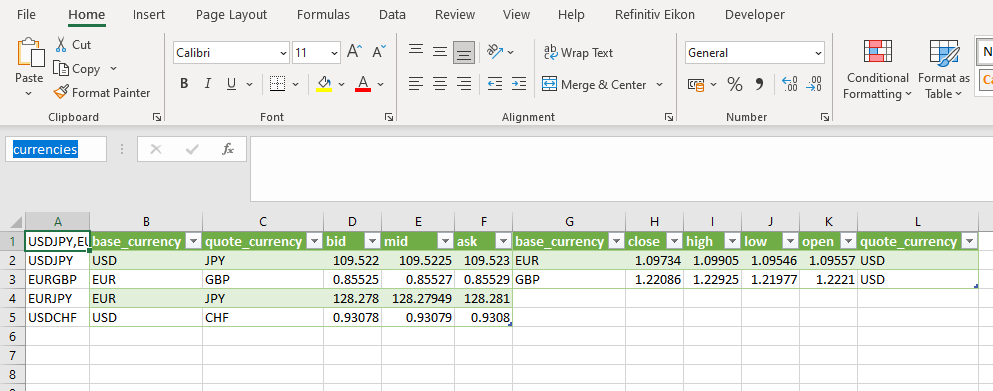
Now click on cell A1 and write "currencies" in the box, as shown below.
Step 11
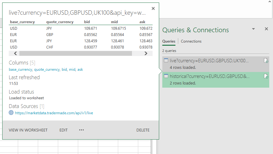
Now right-click on the live query under queries and connections and click EDIT.
Step 12
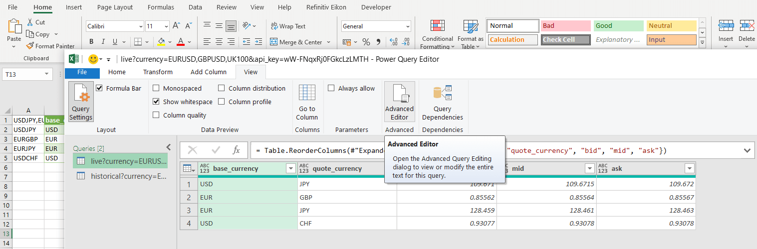
Now Click on the View tab, followed by Advanced Editor.
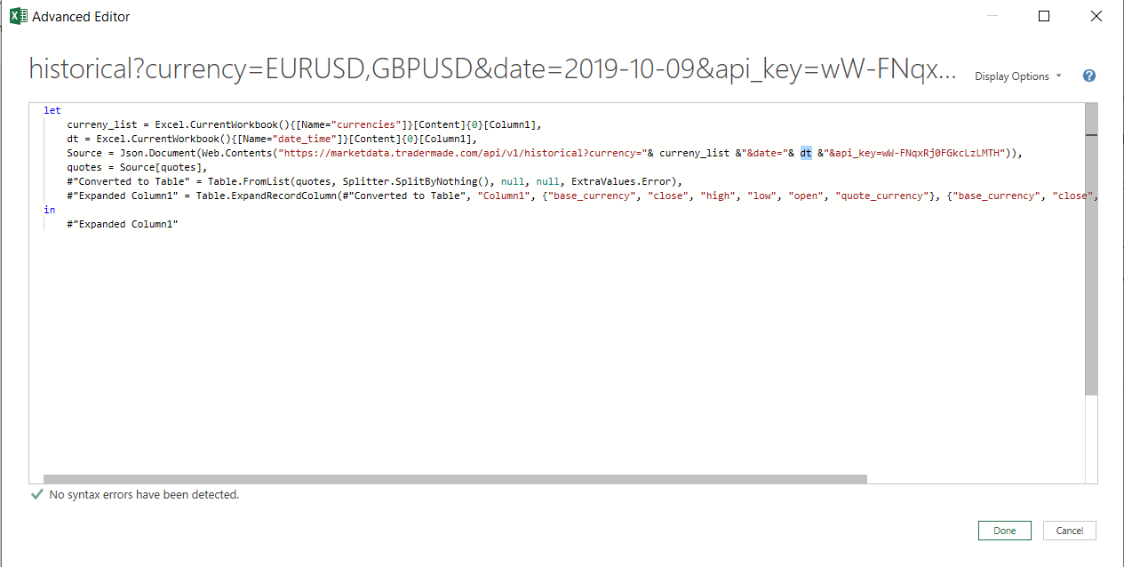
Step 13
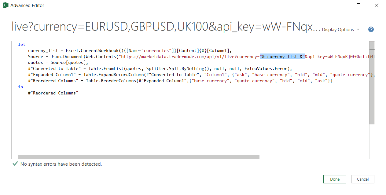
Looking at the image below, it may seem somewhat intimidating (to non-programmers) to alter the code. But don't worry; it's fairly simple. We will define a currency list by the following code:
currency_list = Excel.CurrentWorkbook(){[Name="currencies"]}[ Content]{0}[Column1],
Copy-paste the above line as shown below. The above code gets the data from the excel workbook where the column is named "currencies." Now, change the name of the currencies to "& currency_list &." Then, click done as shown below, followed by closing and loading from the File tab. You will now have live currency rates that you can change from within the spreadsheet.
Step 14
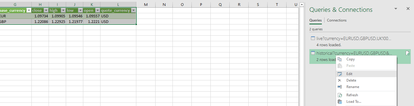
Now, we will change the historical data query to get daily rates for the same currency we requested for live rates. Simple click edit as shown below.
Step 15
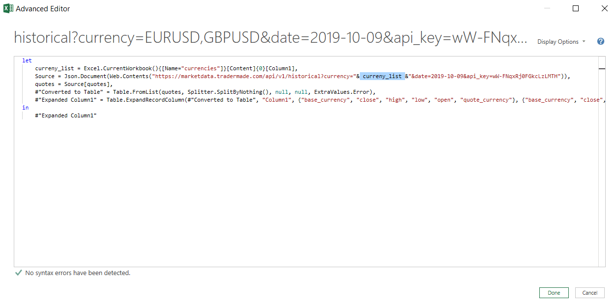
Now click the View tab and click Advance editor as we did in step do the same we did in Step 12. Do the same process as shown below in Step 13, click the "Done" tab and click the Close and load options from the File tab.
Step 16
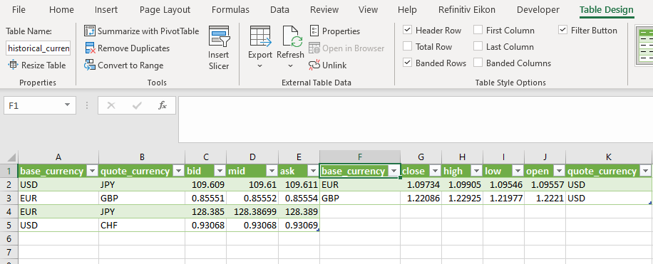
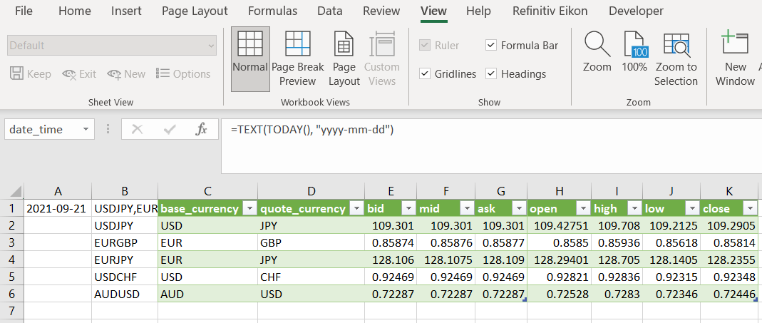
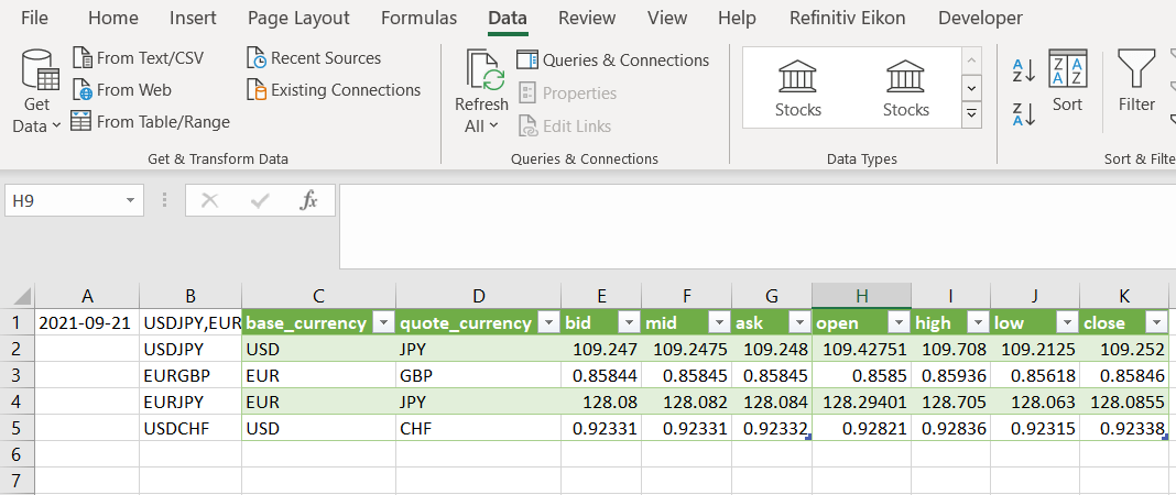
We can now see historical OHLC data updated for the USDJPY, EURUSD, EURJPY, and USDCHF, the same as currencies for live data. However, we have still not set a date we would like to see the historical rates for. If you recollect our initial historical data request in step 2, we requested data for 2019-10-09. What if we wanted to get data for today for all the currencies? Well, let's see how we can do that.
Insert another column and name A1 to date_time and in the cell type, =TEXT(TODAY(), "yyyy-mm-dd") as shown below.
Step 17
Now open Advanced editor by following steps 14 and 15, and this time, We will define a "dt" by the following code:
dt = Excel.CurrentWorkbook(){[Name="date_time"]}[ Content]{0}[Column1],
As we did in step 13, copy-paste the above line as shown below and replace the 2019-10-09 in the url in source to "& dt &" and click "Done."
You can now see we have live and historical rates for the currencies we selected and the date we requested from within the cell.
You can now request rates and refresh data whenever you want. You can set a refresh rate for each query, up to once every minute.
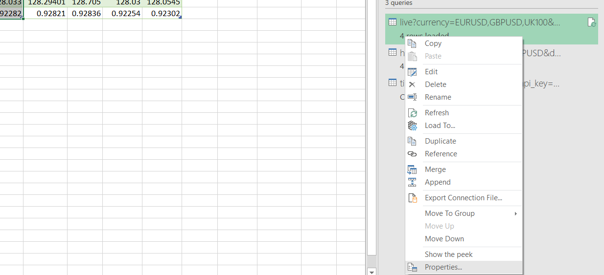
Step 18
Right-click as in the image above, and then set your refresh rate as desired. We have a refresh set every minute, as shown below.
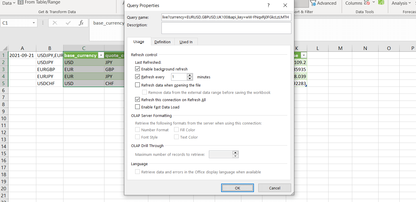
You can refresh as much or as little as you desire. While on a free plan, we recommend refreshing once every hour based on a 12-hour use over 30 days. Do you need a more frequent refresh rate? You can always upgrade your plan from your dashboard. If you have any questions or require assistance, do not hesitate to contact us. We are always open to bespoke requirements.